Technical FAQs

What is the difference between Field Tracing and Classic Field Tracing?

Answering this question requires some brief insights into the history of VirtualLab Fusion. As the name suggests, Classic Field Tracing constitutes an earlier version of field tracing technology. Field Tracing is a more modern, more evolved, better rounded version. From a technical point of view, Field Tracing takes advantage of many theoretical and technological developments that help make physical-optics simulations lighter, faster, more reliable, and more easily controlled by the user:

A hybrid sampling concept that avoids the heaviness of traditional equidistant sampling according to the Nyquist-Shannon sampling theorem.
A more exhaustive and ever-growing list of electromagnetic field solvers which, in practice, means a richer list of available optical components for you to include in your systems.
Flexibility, where those solvers are concerned, in terms of the domain of implementation – the decision is made, on a solver-by-solver basis, on whether the space (x) domain or the spatial frequency (k) domain is more beneficial from a numerical point of view, ensuring that the resulting simulations will be accurate and as fast as possible.
A catalogue of Fourier transform algorithms which not only brings about a huge decrease in the necessary computational resources (both memory and time) in the case of most systems, but which also give the user full control of whether to include diffraction effects in their physical optics simulations – the consideration of diffraction can be switched on and off at will.
A fully unified free-space propagation operator in the k domain coupled with an automatic decision-making process that selects the best candidate from the aforementioned catalogue of Fourier transform algorithms on a case-by-case basis. This all new algorithm replaces the list of historically loaded diffraction integrals used in Classic Field Tracing.
A seamless and flexible framework for non-sequential simulations that allows the user to work with a single system file where the full non-sequential analysis can be simply switched on and off with the use of one button, and even further configured very flexibly for single elements or parts of the system.

Our goal is to phase out the Classic Field Tracing engine step by step. However, some very specific features still only work with Classic Field Tracing – for instance, direct 1D simulations, simulations based on the Fresnel approximation.

How to generate a non-orthogonal (e.g. hexagonal) grating structure?

VirtualLab Fusion always handles the periodization of a grating structure using the reference provided by the x and y directions of an orthogonal coordinate system. This means that, in order to configure a hexagonal array, or a non-orthogonal array in general, as the structure of a grating in VirtualLab Fusion, it is necessary to recalculate, through projection, the values of the periods in x and y, so that a periodic replication of the unit cell thus defined on an x, y grid generates the desired non-orthogonal periodic structure.

The use case “Talbot Images of A Conical Phase Mask” is a perfect example to show that it is possible to define various pillar distributions, including hexagonal, in the form of an array.

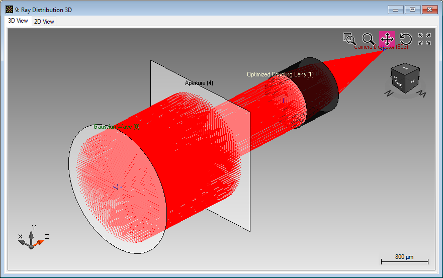
How are apertures handled within 3D ray tracing?

In 3D ray tracing rays are drawn until an aperture blocks them, after which point the rays are no longer drawn for the subsequent parts of the system.

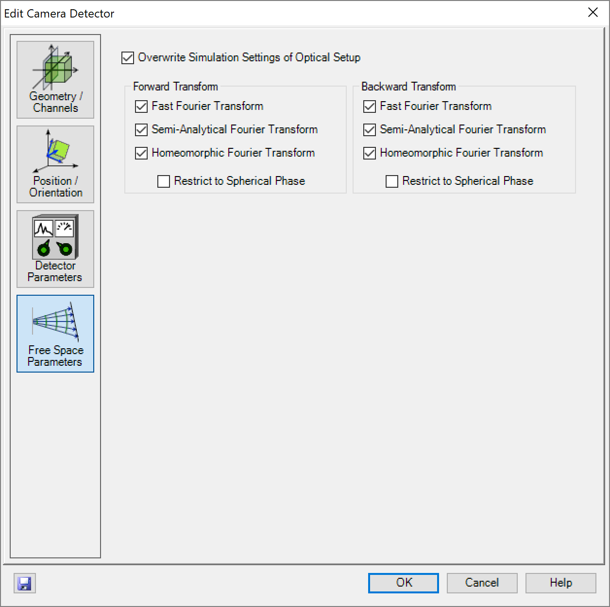
How can I synchronize the settings for the P operator (propagation operator)?

The P operator provides the option to select the types of Fourier transforms that are allowed in the free-space propagation algorithm. Currently the settings can be specified for each propagation step to a detector or component. VirtualLab Fusion envisages the specification per P operator and within the simulation settings of the corresponding optical setup. So you can easily specify the settings within the optical setup settings, or override the system configuration by activating the corresponding option in the detector or component edit dialog.

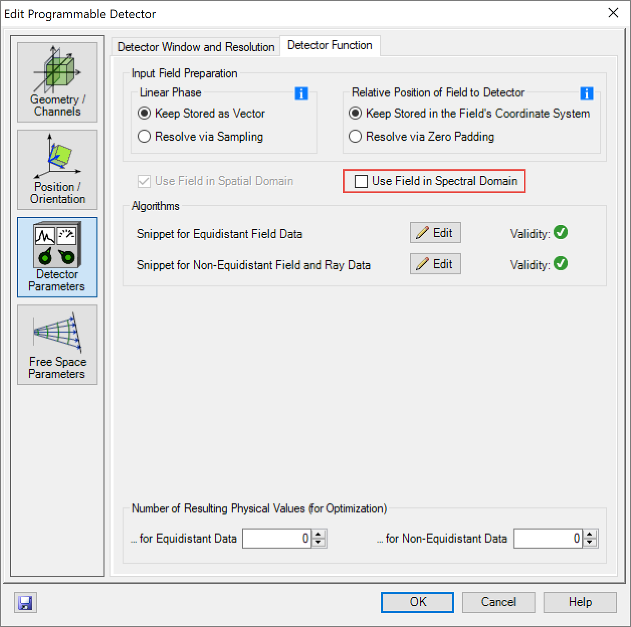
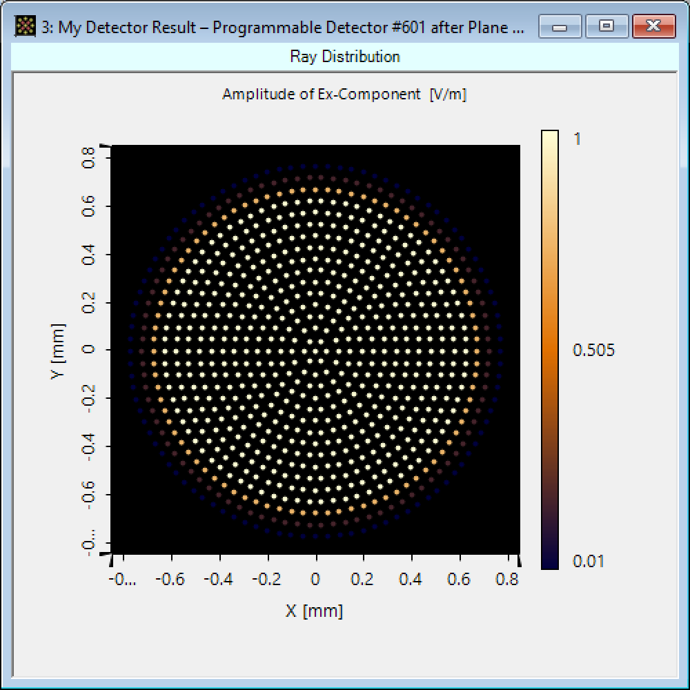
How can I visualize the raw (non-equidistant) field data generated by the field tracing engine?

In former versions of VirtualLab Fusion the raw data container displayed the non-equidistant field data when the detector was placed in the homeomorphic zone of a field. This functionality has been disabled since the 2019 summer release of VirtualLab Fusion. To enable the visualization of the aforementioned raw data, the programmable detector (in its default implementation) can be used. Therefor simply add a programmable detector to your system, at the location where you want to see the field. Then edit the programmable detector and deactivate the option “Use spectral field” (optionally you can also specify to use only homeomorphic (direct and inverse) Fourier transforms).

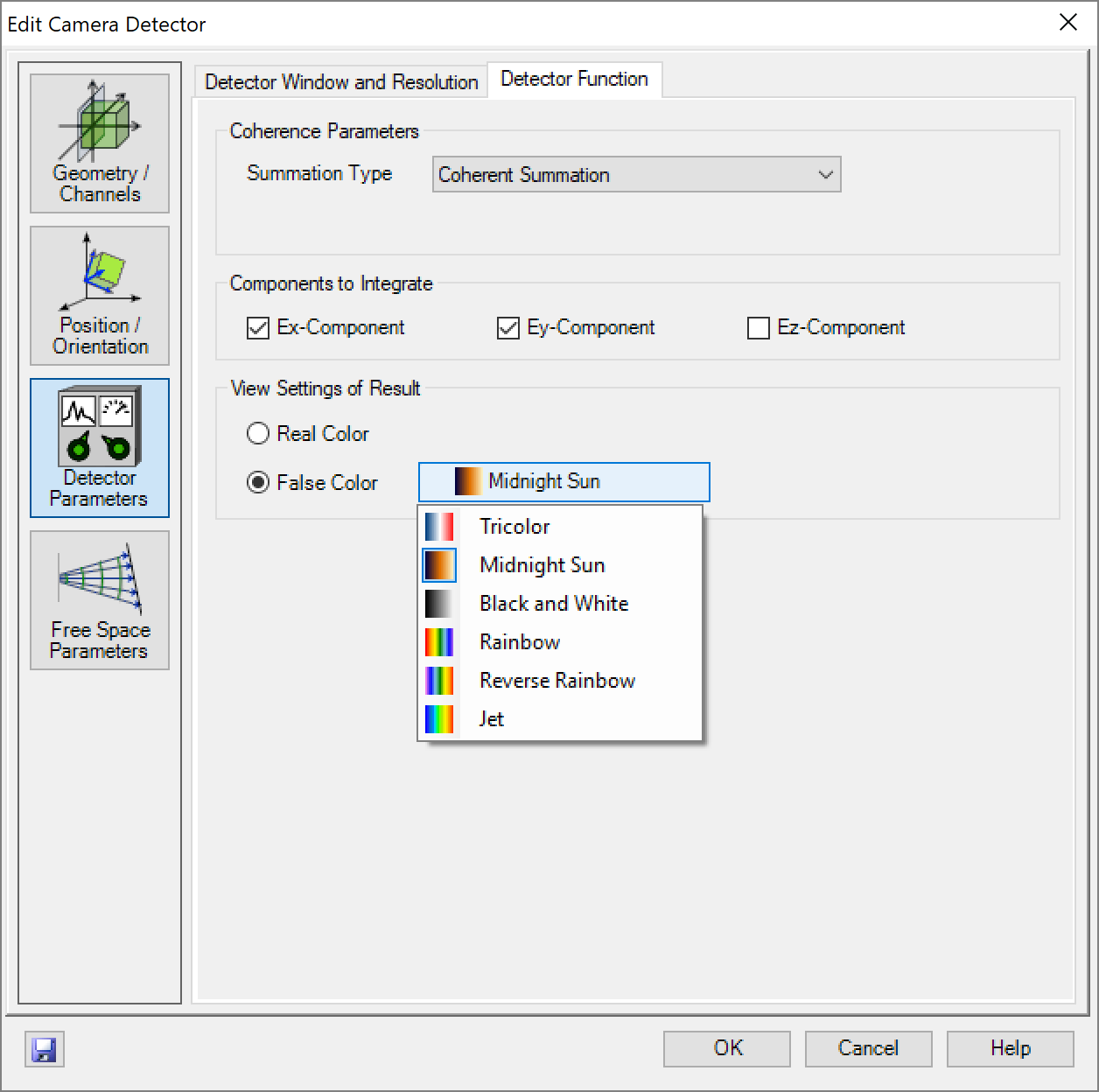
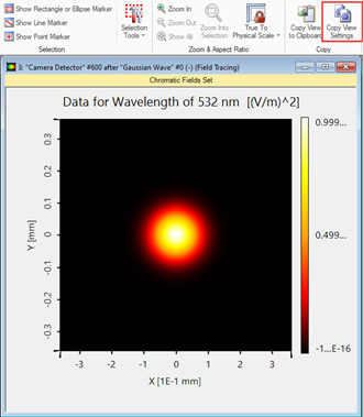
How does VirtualLab Fusion handle the real color visualization (in the camera detector) for wavelengths that are out of the visible range?

The camera detector can be used to calculate the energy density distribution for the incident field. The result is displayed by a chromatic fields set, which provides a real and a false color display. If a wavelength which falls outside the visible range is present in the spectrum, VirtualLab Fusion will switch automatically to the false color mode and log a message in the message window.

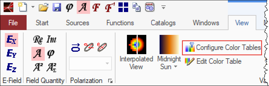
How to configure standard color tables within VirtualLab Fusion?

For the visualization of 2D data VirtualLab Fusion provides a series of predefined color tables. With the VirtualLab Summer Release 2019 you have the option to configure new ones and add them to the predefined list. You simply have to click on the corresponding button in the view ribbon next to the selection of the color table currently used for visualization.
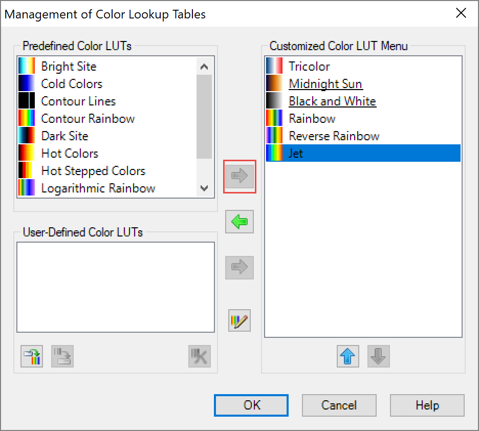
You can select the color lookup tables for the color menu and import user defined color tables. In addition, the selection for the color table menu also has an influence on all those instances where color tables can be selected (e.g. within the camera detector).

Does VirtualLab Fusion support importing Zemax/Code V optics system?

Sequential Zemax Systems: Full support of the import. We are working on that together with Zemax. In VirtualLab Fusion the imported system can be modelled by ray tracing and physical optics, sequentially or with any level of non-sequential modeling.
Non-sequential Zemax Files: No automatized import for non-sequential systems from Zemax.
Code V: No direct automatized import for CODE V systems, but via Zemax only.

Does VirtualLab Fusion support the configuration and analysis of a multiplex grating model?

We enable virtually any kind of stacks for gratings. The gratings may be even on a curved surface for tolerancing or design. Have a look at our use case "Configuration of Grating Structures by using special Media".

Why is the wavelength set in the IFTA document different than the wavelength specified in the session editor?

Actually for the design and optimization of a DOE’s transmission function the wavelength and the subsequent material is required. But the IFTA document does not provide any specification of a material. Instead, it assumes always the vacuum wavelength, and vacuum as subsequent material.
If a design should be done for any other material, it is only necessary to enter the material wavelength λ_material instead of the vacuum wavelength λ_vac. (as opposed to the case of e.g. sources in VirtualLab Fusion, where the wavelength specified is always the one in vacuum, even if the subsequent medium is a different one).
If an IFTA document is preset with the help of a session editor, all the specified parameters are automatically set accordingly, and consequently the vacuum wavelength is also converted to the material wavelength.
Example:
- vacuum wavelenght λ_vac. = 532 nm
- subsequent material = "air" with refractive index n_air (λ_vac.) = 1.000273
  ⇒ the only parameter needed in the IFTA document is:
  λ_air= λ_vac./ n_air = 532 nm / 1.000273 = 531.855 nm
In the optical setup document (OS file), which is also generated by the session editor, VirtualLab Fusion has already preset all parameters according to the specifications entered in the session editor. But if the user presses the button “Show Optical Setup“ in the Analysis tab of the IFTA document, the resulting optical setup document will only exhibit the information known by the IFTA document.
Thus for the above example, the source will be constant with the assumed vacuum wavelength of 531.855 nm and the subsequent material will be vacuum. The user should bear in mind that, if they directly use the IFTA document, they will have to make some manual adjustments.

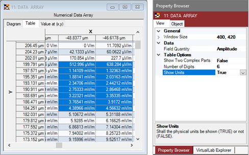
How can I copy a selection of a numerical data array table without units, in order to paste it somewhere else?

In the Property Browser, VirtualLab Fusion offers the flag parameter “Show Units”, which can be set to true or false.

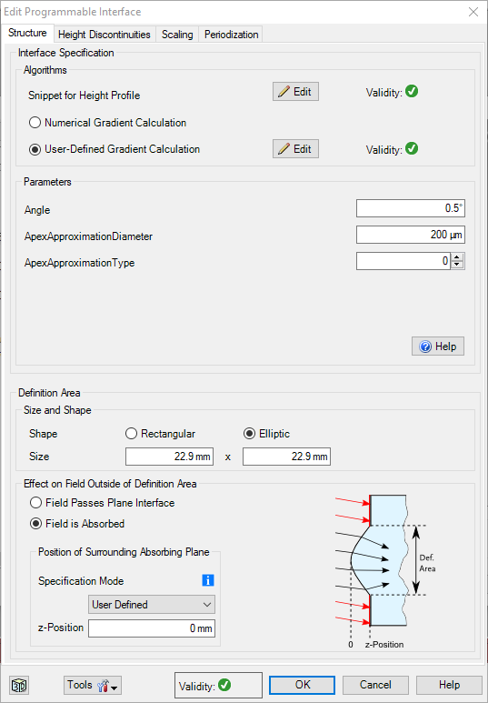
Does VirtualLab Fusion support the import of user-defined surfaces from OpticStudio?

VirtualLab Fusion supports the import of OpticStudio setups. With this import mechanism, several standard surfaces are automatically converted into VirtualLab optical interfaces (see manual for details). The import of custom surfaces defined in Zemax is, however, not supported. Nevertheless, it is possible to define any height profile by a user defined formula in VirtualLab using snippets within the programmable interface. This technique provides a user-friendly way to realize your specific optical interface which is fully embedded in the framework of the VirtualLab user interface (like using parameter run, parametric optimization, …). The programmable interface even supports the user by generating a customized graphic user interface automatically.

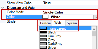
How to make the rays invisible in the 3D ray tracing view?

Sometimes you might want to see, in the 3D Ray Tracing View, just the optical setup without any rays. This can be achieved by making the rays transparent via the Property Browser:

Why are the detector results of a Programmable Detector not shown in a Parametric Optimization as a I programmed them?

Assume you have defined a Programmable Detector which calculates the “Average Efficiency”. Then you want to start a Parametric Optimization and on the Constraint Specification page you wonder that there is only “Value #1”, not “Average Efficiency”, for your Programmable Detector.
The reason for this behavior is that the name of the detector result is only known after the snippet has been executed. And it might be that the execution of the snippet takes some minutes: we have no idea how complex the calculations you have programmed in your snippet are. Thus, we have chosen our implementation so as to not execute the snippet when the Parametric Optimization document is first created, in order to prevent an unforeseen and unnecessary (and possibly long) lag time.
However, you can trigger the execution of the snippet by pressing the Update button on the Constraint Specification page. Then “Value #1” turns into “Value #1: Average Efficiency”.
For the same reason, you must specify the Number of Resulting Physical Values in the edit dialog of the Programmable Detector. If you enter fewer than the real number of physical values generated by your snippet, you cannot optimize all results. If you enter too large a number, the “superfluous” results will always be evaluated to “NaN” and the optimization will fail.
The same mechanism is used for programmable analyzers like the Programmable Grating Analyzer.

For the Far Field Source, the size of the light distribution does not match the size of Source Plane specified in the edit dialog. Why?

We speak here of two different planes, the source plane and the input plane.

The distinction is easily illustrated with a spherical wave generated by a point source: the emitting point is located at the source plane, the plane where the field is actually generated in the system is the input plane (the mathematical singularity of the point source means the two cannot coincide in this case).
In the case of the Far Field Source, each mode starts in the source plane as a spherical wave multiplied by a weighting function D(ϑ, φ) (which can be defined via Programmable Input / Databased Input). In the input plane (where the actual field is generated) the mode is then cut to a certain size – the Diameter of the input field specified on the Basic Parameters tab which, in other words, defines the size of the aperture applied on the complete field in the input plane.

In a Programmable Component, how to mark a ray as absorbed?

If in the Snippet for Non-Equidistant Field and Ray Data you want to set a ray as absorbed, it might seem like a good idea to set, for example, its field scaling matrix to zero (ray.FieldScalingValues = new Matrix2x2C(0);). However, in that case these rays would still be propagated through the system, which artificially degrades performance and can lead to strange effects (e. g. wrong field sizes). Setting the position of the ray to undefined means it is internally treated as really absorbed (ray.Position = Vector3D.UndefinedVector;).

Why does my Programmable Detector not work as intended in Parametric Optimization?

First ensure that the snippet of your detector returns one and only one list of physical values as a result. Take care that the right snippet is executed during your simulations. Furthermore, for technical reasons, the number of physical values made available for parametric optimization must be specified in the edit dialog of the detector. If this number is lower than the actual number of physical values in the detector results, then not all the physical values delivered by the detector will be available as merit function constraints. In contrast, if this number is larger than the actual number of physical values in the detector results, the resulting target function might be non-computable and thus the parametric optimization might fail.

Coordinate Ranges are shown with strange brackets. Why?

In the Property Browser of Data Array based documents you may notice square brackets around the coordinate ranges shown, e.g. “[-250 µm; 249.02 µm[“. This indicates that the lower bound is included in the range, but the upper bound is not. More details you can find in Wikipedia.

The exclusion of the upper coordinate is derived from the convention we made for the nearest neighbor interpolation method to work:

In the nearest neighbor interpolation, every single coordinate has to belong to exactly one sampling point, its nearest neighbor. Consequently, we stipulate that the lower boundary of the coordinate range of one sampling point is inside while its upper boundary is outside that interval. Otherwise we would get into trouble in the following example: Sampling point i has the coordinate 1 mm and sampling point i+1 has the coordinate 2 mm in an equidistant data array with 1 mm sampling distance. Now we need to interpolate the value at coordinate 1.5 mm via nearest neighbor interpolation. If the sampling points’ intervals were closed at both boundaries, it would be impossible to tell where to get the interpolated value from. But due to our definition it is clear that the point 1.5 mm belongs to sampling point i+1 rather than to i.
If we consider the last sampling point in the data array now, its interval’s upper boundary doesn’t belong to the sampling point, so it’s consequent that the upper boundary doesn’t belong to the coordinate range of that data array at all.

Why does VirtualLab Fusion not use all my processor cores?

To answer this question in depth, we need to go into the details of how a processor works, so we made a separate document for this purpose.

How to make result documents look similar?

For documentation purposes it is often required to generate screenshots of simulation results which have the same scaling, font size, etc. In terms of the pre-configuration of result windows, VirtualLab Fusion offers for most settings the possibility to define them in the corresponding detectors or analyzers. Pre-configuration is not supported for some options, however, like font size of labels. We recommend the following workflow to synchronize all screenshots for your documentation:

Perform your simulation once and configure the resulting document as you like.
Keep the well-defined result open (additionally you can also save it to hard disc, view settings should be stored automatically).
After you perform another simulation (e.g. with different settings/geometry) apply the “Copy View Settings” tool on the new result window. The view settings will be automatically synchronized.

Note: The procedure can be performed for all result windows, e.g. 2D results, 1D results and even 3D ray tracing results.

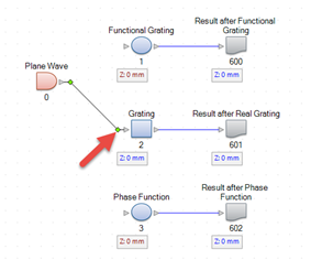
How to configure an optical setup with alternative configurations?

In some situations a user might want to compare the results of an optical setup using different configurations (e.g. using a phase function instead of a height profile). The optical setup view of VirtualLab Fusion supports such kind of situations in a sophisticated way. It is possible to build up both (or even more) configurations within one setup. By changing the connection from the active source to the first element to the other “path”, the user can switch between the different configurations with one click (drag & drop). The same procedure is valid in the middle of the system, should the first elements in the system be the same for all configurations. Especially during live demonstrations for your coworkers this is an efficient way of discussing different situations.

Note: To copy elements in the optical setup view you simply need to mark the element which you would like to copy and press CTRL while doing drag & drop inside the flow chart. After the copy action is done, you simply need to establish the connections between the copied elements.