

Field Tracing Accuracy Settings
Author: Frank Wyrowski (July 22, 2021)
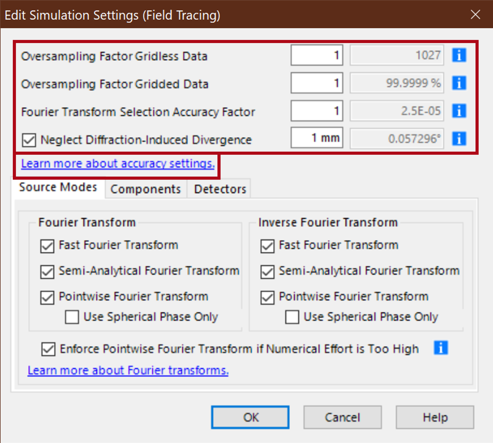
The numerical accuracy of physical optics simulations is controlled by the numerical parameters of each solver, the sampling accuracy of the fields, and the accuracy of the usage of the pointwise Fourier transform. The solvers are discussed in the component dialogs. Here we focus on the accuracy of sampling and the Fourier transform selection. They can be adjusted in the major Simulation Settings (Field Tracing) in each modeling level and in the customized mode of field tracing
Sampling of Electromagnetic Fields
We use a hybrid sampling concept in VirtualLab Fusion to enable fast physical optics modeling. Electromagnetic fields come with six field components, whereby the three magnetic field components are calculated on demand only. Each field component is represented by a complex amplitude. A part of it is sampled and interpolated on an equidistant grid according to sampling theory and we obtain gridded data.
Another part, the wavefront phase which is common to all field components, is sampled on a two-dimensional point cloud and we obtain gridless data. Resampling and changes of the mix between gridded and gridless data are routine key techniques in fast physical optics modeling in VirtualLab Fusion.
Gridless Field Data
In all situations in which gridless data is generated, we use initial sampling positions on a Cartesian grid or a hexapolar grid dependent on the shape of the domain of the complex amplitude, e.g., a circular domain shape leads to a hexapolar grid. Though the initial positions are on a grid, the positions are changed by subsequent operations without restrictions in gridless data. The number of sampling values used in the gridless data initialization can be adjusted by Oversampling factor Gridless Data. The grey box behind the factor provides the information of the sampling number used.
The sampling factor is multiplied on the initial number per direction in case of a Cartesian initial grid. For a hexapolar grid there is no simple linear rule. Thus, it is best to adjust the number interactively by considering the effect on the sampling value number in the grey box when selecting a specific factor. If you see in the modeling, that the wavefront phase or the complex amplitude show some artifacts, try first to increase the factor for gridless data! We work on an additional automatic sampling feature for gridless data, and it will be released in near future.
Gridded Field Data
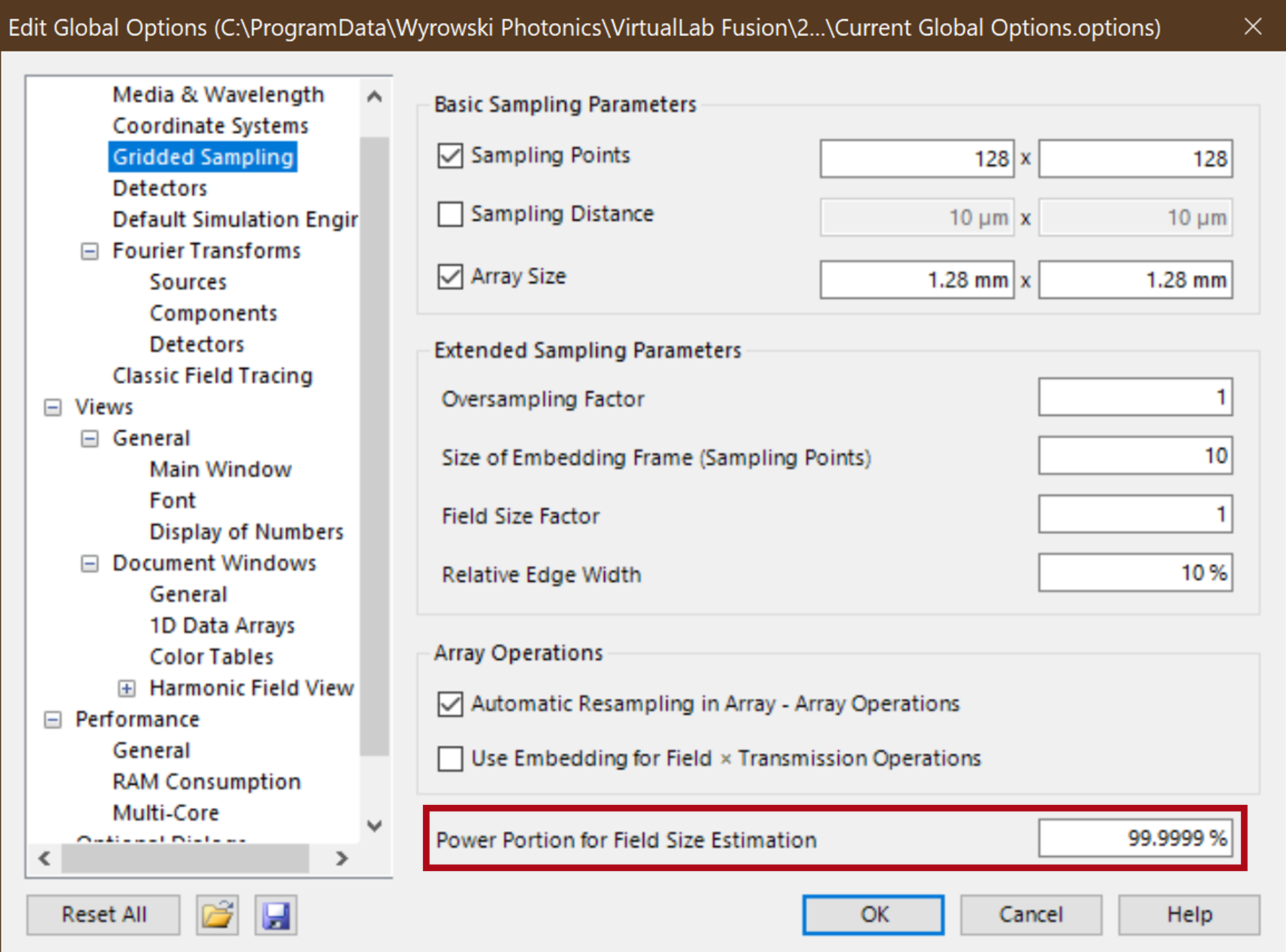
The periods in the x and y direction of an equidistant sampling grid are determined automatically in VirtualLab Fusion for any complex amplitude. According to the sampling theory we calculate the bandwidth of a complex amplitude to conclude the sampling period. In practice we perform several 1D FFTs of selected lines out of the 2D function to estimate the bandwidth. The bandwidth is defined by the size of the data window in the transformed domain in which x% of the square sum of the entire data field is contained. As default we use 99.9999 % which can be adjusted in the Global Options.
The value is also displayed in the grey box in the line Oversampling Factor Gridded Data. From the bandwidth estimation VirtualLab Fusion calculates the Nyquist sampling distance. A value of one of the Oversampling Factor Gridded Data means sampling with the Nyquist distance. A smaller value than one of the oversampling factor results in a sampling period larger than the determined Nyquist distance and vice versa. The default settings in VirtualLab Fusion are well calibrated. However, if results show some numerical artifacts, first increase the number of gridless data points and then, if still needed, the oversampling factor of gridded data. On the other hand, you may try to increase the modeling speed by another compromise between sampling accuracy and speed by reducing the sampling accuracy. The first choice should be a reduction of the default 99.9999 % to say 99.999 % in Global Options. Then, reducing the sampling factor could be tried.
Selection of Fourier Transform
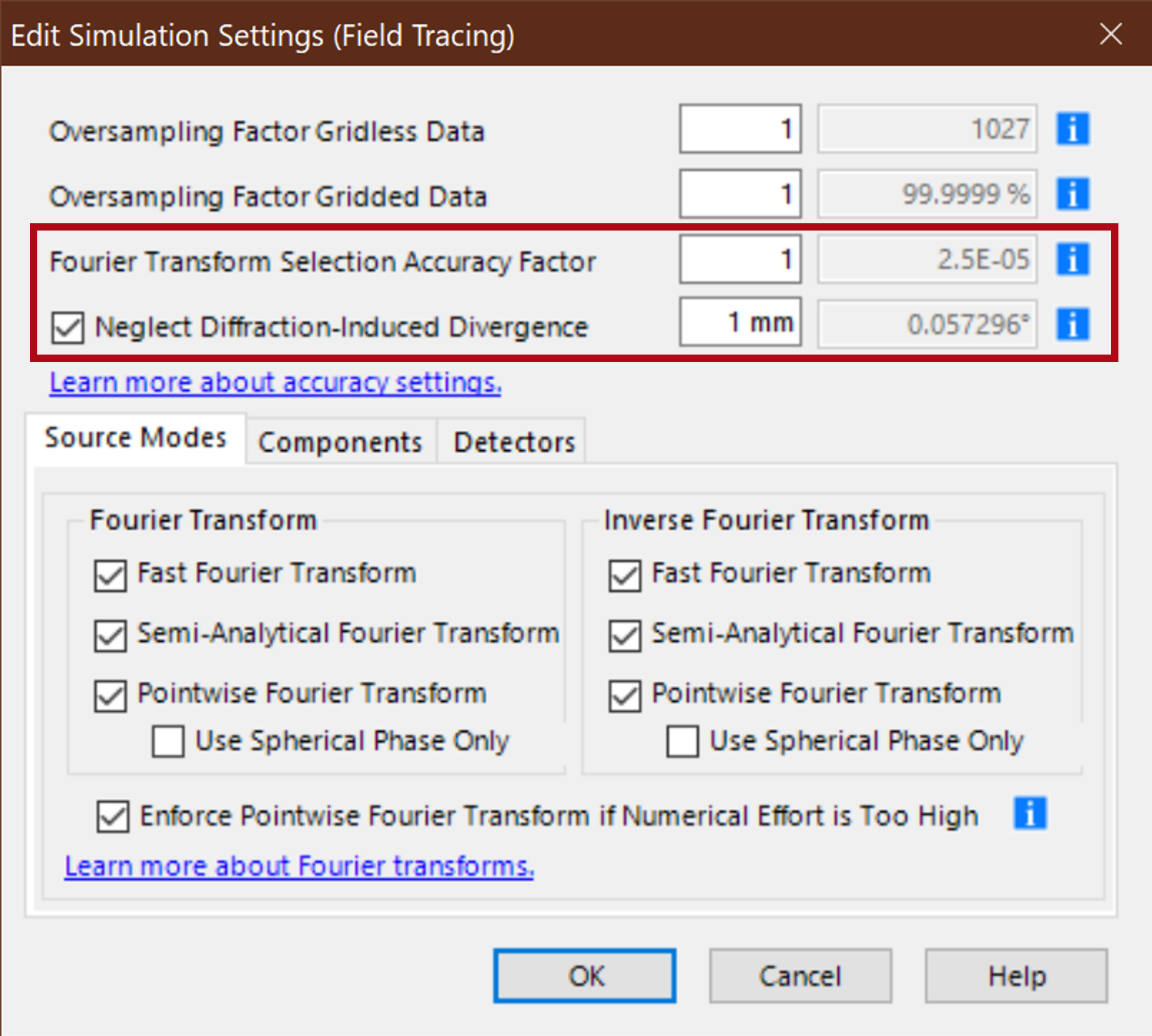
Switching between an integral Fourier transform and a pointwise Fourier transform [Wang 2020] is a key technology in VirtualLab Fusion. See also the White Papers on Seamless Transition from Ray to Physical Optics and Controlling of Fourier Transforms. Here we like to briefly discuss the control Fourier Transform Selection Accuracy Factor and the option Neglect Diffraction-Induced Divergence.
Relative Diffractive Power
Before a complex amplitude is Fourier transformed, its relative diffractive power is determined, which can be understood as the generalization of the Fresnel number. The integral Fourier transform is used if the relative diffractive power is larger than one and the pointwise Fourier transform otherwise. The relative diffractive power is calibrated with respect to the error with which the radius of curvature of a Gaussian beam is calculated when the pointwise Fourier transform is used.
The default error is given in the grey box in the line of Fourier Transform Selection Accuracy, that is 0.0025 %. This value can be adjusted by the value of Fourier Transform Selection Accuracy. Smaller values result in a more frequent use of the pointwise Fourier transform and by that higher speed. Physically it means, that more small diffraction effects are neglected.
Absolute Diffractive Power
Consider the example of a truncated plane wave. The wavefront has no curvature which leads to a relative diffractive power much larger than one. Thus, the integral Fourier transform is used and the diffraction at the boundaries of the plane wave are included during further propagation. On the other hand, if the plane wave diameter is a few millimeters or even centimeters the diffraction effect along a short propagation distance is small. That indicates that the inclusion of diffraction is not always needed or even desired, since it can be a minor effect.
By Neglect Diffraction-Induced Divergence the use of the pointwise Fourier transform can be enforced for such fields with small diffraction effects. As criterion a threshold for the maximum diffraction induced divergence can be selected in terms of mm per meter propagation from which the divergence angle in the grey box follows. If “1 mm” is selected, diffraction effects which cause a spread of a field smaller than one mm per one meter propagation are neglected.
- Z. Wang, O. Baladron-Zorita, C. Hellmann, and F. Wyrowski, ‘Theory and Algorithm of the Homeomorphic Fourier Transform for Optical Simulations’, Optics Express (2020); https://doi.org/10.1364/OE.388022