Define Desired Metalens Functionality
🎬 Overview
As described in the tutorial "Designing a Metalens in VirtualLab Fusion", one possible first step when working with a metalens is to specify the desired phase transformation that the metalens should apply to the incident light.
VirtualLab Fusion 2026.1 (Build 2.8) offers two options for defining a radially symmetric wavefront phase profile:
- Even Order Radial Polynomials – Define spherical, aspherical, or freeform phase profiles using polynomial coefficients (r², r⁴, ...). Coefficients can also be imported automatically from a Zemax OpticStudio Binary 2 surface.
- User Defined Formula – Define the phase profile using a mathematical expression in C# via VirtualLab Fusion's snippet technology.
This tutorial explains this first step in detail. The suggested workflow:
- Configure an optical setup with a light source, the metalens component, and a detector
- Define the wavefront phase profile using one of the two methods
- Verify the optical function using ray tracing
Both methods support parameter optimization – you can automatically adjust coefficients to meet your design goals before continuing with the generation of the surrogate model.
At the end you find two examples with downloadable files that use the User Defined Formula.
🚀 Step-by-Step Tutorial
Step 1: Set Up the Optical System
Before defining the wavefront, you need a basic optical setup to test your metalens functionality.
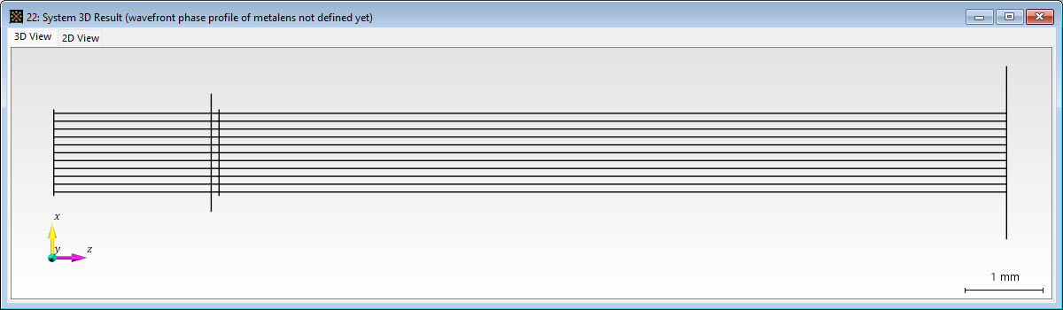
Let us assume a simple case: a plane wave illuminates the metalens, and we want to see the result on a detector 1 mm behind the metalens.
Procedure:
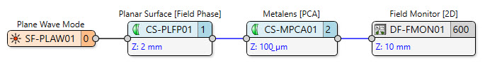
- Open a new optical setup (File → New → Optical Setup)
- Insert the following components:
- A Plane Wave Mode source (or any illumination matching your intended use)
- A Planar Surface [Field Phase] for the substrate
- A Metalens [PCA] component
- A Field Monitor [2D] detector
- Connect the components in the order listed above
- Configure the distances:
- Set the distance between the substrate and metalens surface to 100 µm
- Set the distance between Metalens and Detector to 10 mm
- Configure the light source and surfaces (wavelength, beam and element diameter, etc.) according to your needs (a metalens diameter that is much larger than the beam profile will unnecessarily increase computation time in later steps)
Now you are ready to define the metalens functionality.
💡 Note: You can use Ray Tracing first to quickly verify the wavefront profile before running full field tracing. For a Field Tracing simulation, a surrogate model must first be trained and then bound to the metalens.
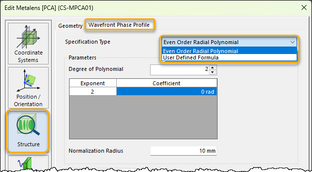
Step 2: Define the Desired Wavefront Profile
To define the wavefront profile for the metalens:
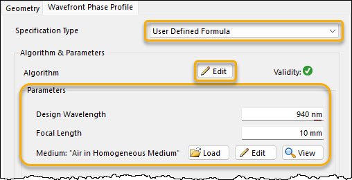
- Open the Metalens [PCA] component's property dialog
- Navigate to the "Wavefront Phase Profile" section under the Structure tab
- Select the desired definition method from the dropdown menu
💡 Important: After performing a field tracing simulation, the wavefront profile becomes locked and cannot be edited. To make changes, delete the existing design first: go to the "Simulation Model" page, delete the design there, then return to adjust the wavefront profile.
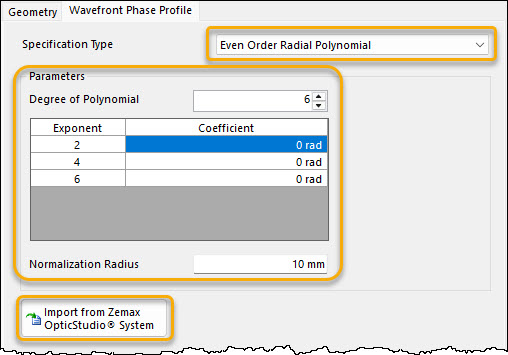
Method 1 – Even Order Radial Polynomials
This method defines the phase profile as a radial polynomial containing only even-order terms:
\(\Phi(r) = \sum_{n=1}^{N} A_n \cdot \left(\frac{r}{r_0}\right)^{2n}\)
where: - \(r\) = radial coordinate - \(r_0\) = normalization radius (reference radius for scaling) - \(A_n\) = polynomial coefficients
The user can either enter the values manually, via a parametric optimization process or by importing a Binary 2 surface from Zemax OpticStudio.
The polynomial coefficients can be treated as optimization parameters. For example, to design a focusing metalens:
- Define a merit function (e.g., minimize spot size at the focal plane)
- Set A₁ (focusing power) as an optimization variable
- Use the parametric optimization document to find the optimal coefficient value
Higher-order coefficients (A₂, A₃, ...) can be optimized to correct spherical aberration or shape the beam profile.
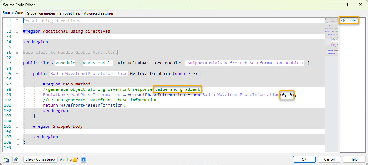
Method 2 – User Defined Formula
The User Defined Formula method provides maximum flexibility. You write a custom 1D formula as a function of the radial coordinate r using VirtualLab's C# snippet technology, e.g., for representing a focusing lens or an axicon (conical lens).
Procedure:
- Select "User Defined Formula" as the definition method
- Click "Edit" in the Algorithm & Parameters section to open the snippet editor
- Write your phase function using
ras the independent variable and define possible additional parameters - Validate the syntax using the "Check" button
Step 3: Verify with Ray Tracing
Before committing to a full field tracing design (which requires a surrogate model), you can quickly verify if your specified wavefront phase profile achieves the desired effect using Ray Tracing. Ray tracing uses only the phase profile and neglects diffraction – it gives you an immediate check of the basic optical function.
- In the main toolbar, click the Ray Tracing button
- Observe the ray paths and spot diagram
- If the result is not as expected, go back and adjust your wavefront phase profile definition
Once you are satisfied, proceed to field tracing and surrogate model training (see the main metalens tutorial "Designing a Metalens in VirtualLab Fusion".
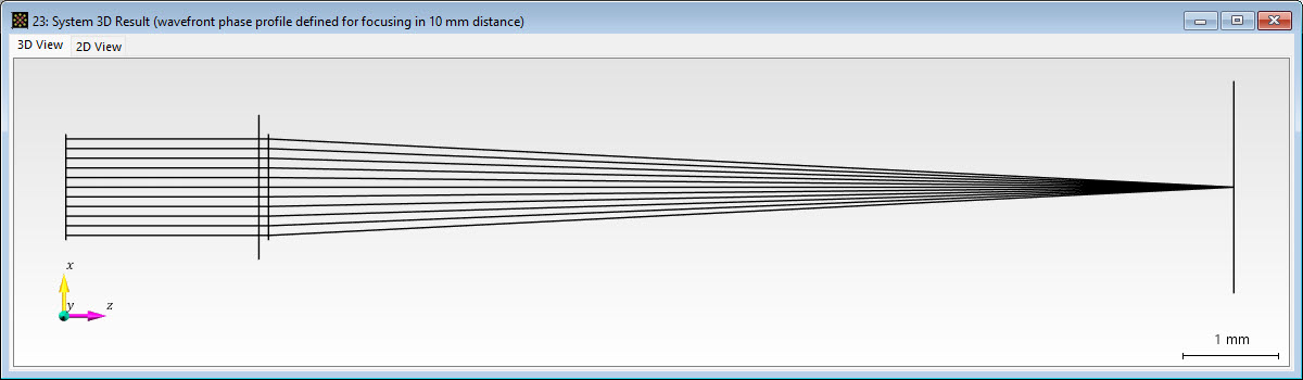
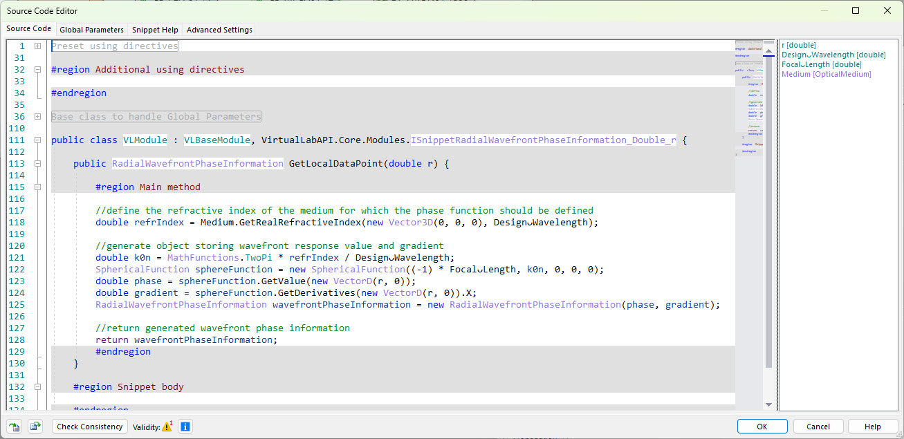
Example 1: Simple Focusing Lens for Collimated Light
Above's shown ray tracing results and the screenshot of the dialog for 'User Defined Formula' with exemplary parameters belong to this example, where we have defined a spherical wavefront phase profile that focuses a plane wave with a focal length of 10 mm:
Downloads of Example 1
- Basic optical setup file
- Optical setup file with the preset user defined spherical wavefront phase profile definition
- Exported code snippet which can be imported to metalens components in other optical setups - Import and export are done via associated buttons at the bottom left of the source code editor.
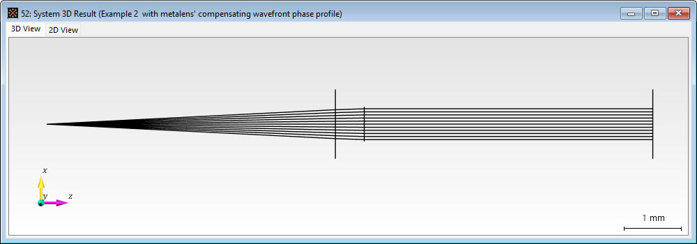
Example 2: Wavefront Compensation
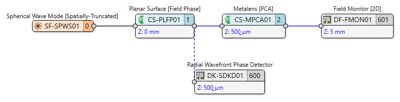
This example shows how to compensate for an unwanted radial wavefront distortion. Here we have a spherical input beam and we want the metalens introducing an inverted wavefront, so that they cancel each other out, thus we expect to receive a collimated beam.
We start again with a basic setup, but this time we include the Radial Wavefront Phase Detector twin, which evaluates the beam's radial wavefront phase profile just in front of the metalens surface. This wavefront phase information is then fed to our Metalens [PCA] component so that the user defined code can generate the inverse.
Thus, the simulation steps are as follows:
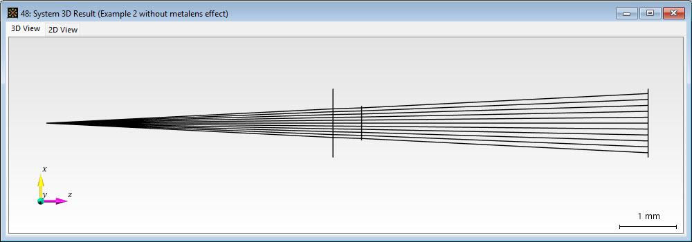
- Do a Ray Tracing System 3D simulation of the basic OS with deactivated Radial Wavefront Phase Detector. This shows us the uncompensated ray illustration.
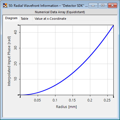
- Do a Ray Tracing Detector simulation with just the activated Radial Wavefront Phase Detector. By that we get the radial wavefront phase curve of the incident beam.
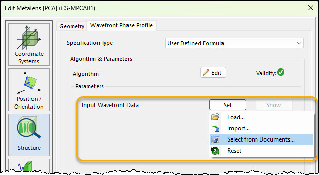
- Set this wavefront phase information in the Metalens [PCA].
- Do a Ray Tracing System 3D simulation with only the Field Monitor [2D] detector and check the effect of the metalens' wavefront phase response function.
Downloads of Example 2
- Basic optical setup file
- Optical setup file with the preset user defined code for compensation of given wavefront phase
- Exported code snippet of this metalens's user defined wavefront phase definition which can be imported to metalens components in other optical setups - Import and export are done via associated buttons at the bottom left of the source code editor.
- Exported code snippet of the add-on used in the Radial Wavefront Phase Detector - Import and export are done via associated buttons at the bottom left of the source code editor.
Important Notes
- Design locking: Once a field tracing simulation runs, the wavefront phase profile becomes locked. To modify it, delete the existing design in the "Simulation Model" page first.
- Ray tracing first: Always use ray tracing to quickly verify your wavefront profile before committing to full field tracing. It saves time.
- Units: Phase values are typically specified in radians (not waves). When importing from Zemax, conversion is handled automatically.
- Radial symmetry: Both methods assume radial symmetry. For non-radially symmetric phase profiles, use other component types or the full programmable interface.
Summary
| Method | Best For | Optimization Support |
|---|---|---|
| Even Order Radial Polynomials | Spherical, aspherical, or freeform profiles; Zemax import | Yes (coefficients) |
| User Defined Formula | Custom shapes, wavefront compensation, complex functions | Yes (user-defined parameters) |
Both methods allow you to:
- Define the desired optical function without full metasurface design
- Quickly test performance using ray tracing
- Optimize parameters automatically
- Later design the actual metasurface using a surrogate model
Last updated: April 22, 2026 Tags: metalens wavefront phase profile response compensate optimization VirtualLab Fusion